
Articles
- Page Path
- HOME > Osong Public Health Res Perspect > Volume 12(3); 2021 > Article
-
Original Article
A spatial analysis of the association between social vulnerability and the cumulative number of confirmed deaths from COVID-19 in United States counties through November 14, 2020 -
Baksun Sung

-
Osong Public Health and Research Perspectives 2021;12(3):149-157.
DOI: https://doi.org/10.24171/j.phrp.2020.0372
Published online: June 2, 2021
Department of Sociology, Social Work, and Anthropology, Utah State University, Logan, UT, USA
- Corresponding author: Baksun Sung Department of Sociology, Social Work, and Anthropology, Utah State University, 0730 Old Main Hill, Logan, UT 84322-0730, USA E-mail: baksun777@gmail.com
• Received: December 30, 2020 • Revised: February 9, 2021 • Accepted: April 13, 2021
© 2021 Korea Disease Control and Prevention Agency
This is an open access article under the CC BY-NC-ND license (http://creativecommons.org/licenses/by-nc-nd/4.0/).
Abstract
-
Objectives
- Coronavirus disease 2019 (COVID-19) is classified as a natural hazard, and social vulnerability describes the susceptibility of social groups to potential damages from natural hazards. Therefore, the objective of this study was to examine the association between social vulnerability and the cumulative number of confirmed COVID-19 deaths (per 100,000) in 3,141 United States counties.
-
Methods
- The cumulative number of COVID-19 deaths was obtained from USA Facts. Variables related to social vulnerability were obtained from the Centers for Disease Control and Prevention Social Vulnerability Index and the 2018 5-Year American Community Survey. Data were analyzed using spatial autoregression models.
-
Results
- Lowest income and educational level, as well as high proportions of single parent households, mobile home residents, and people without health insurance were positively associated with a high cumulative number of COVID-19 deaths.
-
Conclusion
- In conclusion, there are regional differences in the cumulative number of COVID-19 deaths in United States counties, which are affected by various social vulnerabilities. Hence, these findings underscore the need to take social vulnerability into account when planning interventions to reduce COVID-19 deaths.
- Coronavirus disease 2019 (COVID-19) is an extremely infective respiratory ailment, caused by severe acute respiratory syndrome coronavirus 2 (SARS-CoV-2) [1]. The cumulative confirmed COVID-19 death for the United States was 242,431 as of November 14, 2020, which is the highest in the world [2]. The case fatality rate of COVID-19 in the United States was 2.3%, compared to the world average of 2.4% as of November 14, 2020 [3]. The case fatality rate of COVID-19 (2.3%) is higher than that of the seasonal flu (0.1%) in the United States [4]. In addition, SARS-CoV-2 is more contagious than other corona viruses such as SARS-CoV and Middle East respiratory syndrome coronavirus [1] which has led to a public health crisis in the United States.
- Social vulnerability is defined as the vulnerability of a social group to potential damage from hazards [5,6] and the characteristics of a group with regard to its ability to cope with the effects of social and natural hazards [7]. Social vulnerability is influenced by social, economic, demographic, and geographic features, which determine exposure to hazards as well as a community’s ability to cope with hazards [8]. Measures of social vulnerability include socioeconomic status [9–11], disability [12], minority status [13], demographic make-up by age [14,15], race and ethnicity [16,17], housing status [18, 19], family structure [20], social security [21], and public health conditions [22,23].
- Social vulnerability also has a major influence on mortality and health outcomes. Specifically, high social vulnerability is a predictor of mortality [24]. Public health conditions, including access to healthcare are closely related to the health status of a population [22]. Poor public health conditions are generally linked to other measures of social vulnerability such as low socioeconomic status and poor quality of housing [25]. Thus, social vulnerability is deep-rooted in social structures that lead to an unequal distribution of exposure to hazards and create social problems [26].
- Pandemics, such as the COVID-19 pandemic, are considered natural hazards [27], and social vulnerability includes the susceptibility of groups to potential damages from natural hazards [5,6]. Hence, COVID-19 deaths are likely to vary according to levels of social vulnerability. In one study, high social vulnerability was positively associated with a higher rate of COVID-19 deaths in Chicago, IL, USA [8]. However, little is known about the association between social vulnerability and COVID-19 deaths across the United States. Therefore, the objective of this study was to examine the association between social vulnerability and the cumulative number of confirmed COVID-19 deaths (per 100,000) in 3,141 counties in the United States.
Introduction
- Data
- This study analyzed the cumulative number of confirmed COVID-19 deaths over a fixed time period using pre-existing cross-sectional social vulnerability data in counties in the United States. First, to analyze the association between social vulnerability and COVID-19 deaths, the number of confirmed COVID-19 deaths in counties in the United States was obtained from USA Facts [2]. At the time of this study, USA Facts released data on the cumulative number of COVID-19 deaths every day. For this study, the cumulative number of confirmed COVID-19 deaths up to November 14, 2020, was analyzed. The dependent variable (cumulative number of confirmed COVID-19 deaths) was changed to a per capita figure (deaths per 100,000 residents) to minimize the effect of the number of residents in a county on the dependent variable. The cumulative number of COVID-19 deaths (per 100,000) was mapped (Figure 1). The dependent variable was log-transformed to reduce skewness.
- Second, variables related to social vulnerability were obtained from the Centers for Disease Control and Prevention (CDC) Social Vulnerability Index [28] and the 2018 5-Year American Community Survey at the county level [29]. Fifteen high social vulnerability variables (flags) were obtained from the CDC Social Vulnerability Index. Flags are interpreted as follows: “tracts in the top 10%, i.e., at the 90th percentile of values, are given a value of 1 to indicate high vulnerability whereas tracts below the 90th percentile are given a value of 0” [28]. Next, the percentage of people without health insurance and 2 control variables (population and the percentage of male) were obtained at the county level from the 2018 5-Year American Community Survey.
- This study did not require approval from the Institutional Review Board because the datasets were secondary data that did not include personal information.
- Data Analysis
- The ordinary least squares (OLS) regression model assumes that all variables are independent, which ignores potential spatial dependencies that might lead to bias related to potential spatial autocorrelation [30,31]. The fundamental law of geography states that spatial units near to each other are more strongly related, even though every spatial unit is related to everything else [30]. Hence, to control potential bias related to spatial autocorrelation, spatial autoregression models were applied in the study. This is supported by Table 1. A low value of the Akaike information criterion (AIC) indicates that a model is more appropriate; on this basis, the spatial lag and spatial error model were deemed appropriate for use (AIC values: OLS, 10,179.03; spatial lag, 9,806.87; spatial error, 9,754.02).
- First, the spatial lag model states that “outcome in one spatial unit is linked to outcome in another spatial unit” [32]. The main purpose of this model is to correct for spatial dependence by adopting a term for the effect of the spatially lagged Y on Y [31,33]. In other words, the outcome variable in location a is affected by its neighboring location [31,33]. It can be summarized as follows:
- (1) Y is the dependent variable, (2) ρ is the lag coefficient, (3) W is the spatial weight matrix, (4) β is the coefficient for a vector of social vulnerability variables, and (5) ε is the error term.
- Second, the spatial error model states that “unobserved factors in one spatial unit are linked to unobserved factor in another spatial unit” [32]. In other words, the error term in location a is affected by neighboring location b [31,33]. It can be summarized as follows:
- (1) Y is the dependent variable, (2) β is the coefficient for a vector of social vulnerability variables, (3) λ is the coefficient, (4) W is the spatial weight matrix, (5) ε is the residual error matrix, and (6) v is the normal assumption for the error term.
- All Statistical analyses were conducted using STATA ver. 15.0 (StataCorp., College Station, TX, USA).
Materials and Methods
- Tables 2 and 3 shows the descriptive statistics. Counties in the 90th percentile or higher with regard to the following parameters had higher COVID-19 mortality rates than counties below the 90th percentile for the corresponding indicator: (1) the percentage of persons in poverty (mean: 4.292 vs. 3.547 per 100,000 population); (2) the percentage of unemployed persons (mean: 4.045 vs. 3.574 per 100,000 population); (3) per capita income (mean: 4.248 vs. 3.551 per 100,000 population); (4) the percentage of persons with no high school diploma is (mean: 4.279 vs. 3.549 per 100,000 population); (5) the percentage of persons aged 65 and older (mean: 2.917 vs. 3.697 per 100,000 population); (6) the percentage of persons aged 17 and younger (mean: 3.810 vs. 3.600 per 100,000 population); (7) the percentage of persons with a disability (mean: 3.467 vs. 3.638 per 100,000 population); (8) the percentage of single parent households (mean: 4.437 vs. 3.532 per 100,000 population); (9) the percentage of minorities (mean: 4.329 vs. 3.543 per 100,000 population); (10) the percentage of those with limited English proficiency (mean: 4.094 vs. 3.568 per 100,000 population); (11) the percentage of households in multi-unit housing complexes (mean: 3.823 vs. 3.599 per 100,000 population); (12) the percentage of mobile home residents (mean: 4.172 vs. 3.560 per 100,000 population); (13) the percentage of crowded households (mean: 3.907 vs. 3.591 per 100,000 population); (14) the percentage of households with no vehicles (mean: 4.111 vs. 3.568 per 100,000 population); and (15) the percentage of persons in institutionalized group quarters (mean: 3.665 vs. 3.616 per 100,000 population).
- Table 1 shows the results of regression models for social vulnerability and the cumulative number of COVID-19 deaths. The results of the OLS regression model were generally similar to the spatial lag model and spatial error model, but it overestimated the outcome of the percentage of crowded households in the 90th percentile (OLS, –0.253**; spatial lag, –0.134; spatial error, –0.115).
- Unstandardized coefficients from the spatial autoregression models indicated that counties in the 90th percentile or above for the following parameters showed significant associations with COVID-19 death rates compared to their counterparts: (1) per capita income (spatial lag: B=0.216, p<0.05; spatial error: B=0.221, p<0.05); (2) the percentage of persons with no high school diploma (spatial lag: B=0.280, p<0.01; spatial error: B=0.286, p<0.01); (3) the percentage of persons aged 65 and older (spatial lag: B=−0.254, p<0.001; spatial error: B=−0.285, p<0.001); (4) the percentage of persons aged 17 and younger (spatial lag: B=−0.170, p<0.05; non-significant results for the spatial error model); (5) the percentage of persons with a disability (spatial lag: B=−0.172, p<0.05; non-significant results for the spatial error model); (6) the percentage of single parent households (spatial lag: B=0.303, p<0.001; spatial error: B=0.165, p<0.05); (7) the percentage of households in multi-unit housing complexes (spatial lag: B=−0.172, p<0.05; spatial error: B=−0.350, p<0.001); (8) the percentage of mobile home residents (spatial lag: B=0.266, p<0.01; spatial error: B=0.302, p<0.001); (9) the percentage of persons without health insurance (spatial lag: B=0.032, p<0.001; spatial error: B=0.034, p<0.001).
- The log likelihood ratio (spatial lag, 9,764.87; spatial error, 9,712.02) and AIC (spatial lag, 9,806.87; spatial error, 9,754.02) were lower for the spatial error model, implying that it would be more appropriate. However, both models were used herein because the differences between the 2 models were not major.
Results
- This study found that low income and low educational levels were positively associated with a higher cumulative number of COVID-19 deaths. Economic hardship has been associated with the risk of mortality [34–36]. In 2000, Mirowsky et al. [37] showed that, for populations below the 20th percentile for income, the risk of mortality rose increasingly sharply closer to the lowest levels of income. People with a low education level tend to experience economic hardship since they are more likely to work part-time or be unemployed than those with high education levels [37]. In addition, a low educational level decreases one’s sense of personal control over health behaviors, which could lead to poor health outcomes [37]. However, health literacy—that is, the ability to understand health information—can mitigate the positive effect of a low educational level on poor health behaviors [38]. Therefore, providing poorly educated people with health education related to COVID-19 prevention would be a good way to reduce COVID-19 deaths.
- This study also found that a positive association between a county’s proportion of single parent households and a high cumulative number of COVID-19 deaths. Previous studies have reported that single parenthood has a negative effect on the health status of families due to economic hardship [39,40]. In the United States, single mothers are more likely to live in poverty than 2 parent families due to the difficulties single mothers face working and childrearing at the same time [41]. These conditions could lead to a higher cumulative number of COVID-19 deaths among single parent households.
- Additionally, this study found that a positive association between the proportion of mobile home residents in a county and a high cumulative number of COVID-19 deaths. Mobile homes are concentrated in rural counties with high poverty rates since people with low income are more likely to live in mobile homes than those with high income [42]. This might explain the high cumulative number of COVID-19 deaths in counties with a percentage of mobile homes in the 90th percentile or above.
- This study also found a positive association between a high percentage of people without health insurance and a high cumulative number of COVID-19 deaths. Health insurance helps people obtain access to health care by reducing the cost of medical services. Hence, uninsured Americans are at a higher risk of mortality since they are less likely to receive proper treatment for medical conditions [43,44]. This could lead to higher cumulative number of COVID-19 deaths in counties with a high proportion of uninsured people. America has an employment-based health insurance system that results in many unemployed and self-employed people lacking health insurance due to expensive health insurance premiums. In 2018, 8.5% of the United States population (27.5 million people) did not have health insurance [45]. In addition, hospitals were already operating beyond their capacity after a huge influx of patients and people with COVID-19, limiting access to healthcare services for those with and without insurance. Hence, public health authorities need to provide uninsured people with affordable health insurance as well as tools and education for COVID-19 prevention. Carefully designed guidelines for preventing COVID-19 or mass media campaigns that emphasize its dangers and the expected health benefits of prevention may contribute to reducing the number of COVID-19 deaths.
- United States policymakers have focused on reducing welfare and encouraging work since the 1980s, through policies influenced by neo-liberalism. Given this trend, the United States welfare system today consists largely of a work-based safety net, containing elements such as the Earned Income Tax Credit [41,46]. Although Americans have achieved economic prosperity through capitalism and the free economy, the U.S. also has many social problems such as a large wealth gap between the rich and the poor, a socially vulnerable class, a high uninsured rate, and a high mortality rate for vulnerable populations. As shown in Figures 1 and 2, the counties with the highest rates of COVID-19 deaths roughly correspond to counties with the highest social vulnerability indices, in areas such as: (1) northeastern Arizona, southeastern Utah, and northwestern New Mexico (Indian reservation); (2) western Kansas, western Texas, and southern Texas; (3) Louisiana, Mississippi, Alabama, Georgia, South Carolina, and Florida (corresponding to the American South); (4) eastern Washington, eastern Oregon, Idaho, and Montana (corresponding to the Inland Northwest region); (5) South Dakota, and North Dakota; and (6) New York City, Newark, and Jersey City (corresponding to the NY-NJ-PA metropolitan statistical area). Therefore, it is necessary to strengthen the social safety net to reduce COVID-19 deaths in the most vulnerable populations.
- The observations of this study should be considered in light of several limitations. First, the temporal causal relationship between social vulnerability and the cumulative number of COVID-19 deaths cannot be determined due to the cross-sectional study design. Second, the log-transformed dependent variable may hide real variations in the rate of COVID-19 deaths in United States counties. Third, this study used pre-existing cross-sectional social vulnerability data from 2018 that may not coincide with data on COVID-19 deaths through November 14, 2020.
Discussion
- Despite these limitations, this study conducted a spatial analysis of the association between social vulnerability and the cumulative number of COVID-19 deaths in counties in the United States and discovered. There are regional differences in the cumulative number of COVID-19 deaths that were affected by various social vulnerabilities. Low income and low education levels, as well as a high percentage of single parent households, mobile home residents, and people without health insurance, were positively associated with a high cumulative number of COVID-19 deaths. Hence, these findings underscore the need to take social vulnerability into account when planning interventions to reduce COVID-19 deaths.
Conclusion
-
Ethics Approval
Not applicable.
-
Conflicts of Interest
The author has no conflicts of interest to declare.
-
Funding
None.
-
Availability of Data
All data generated or analysed during this study are included in this published article. For other data, these may be requested through the corresponding author.
Article information
Figure 1.Mainland United States map of cumulative number of confirmed deaths from coronavirus disease 2019 (per 100,000 population) by county level through November 14, 2020.
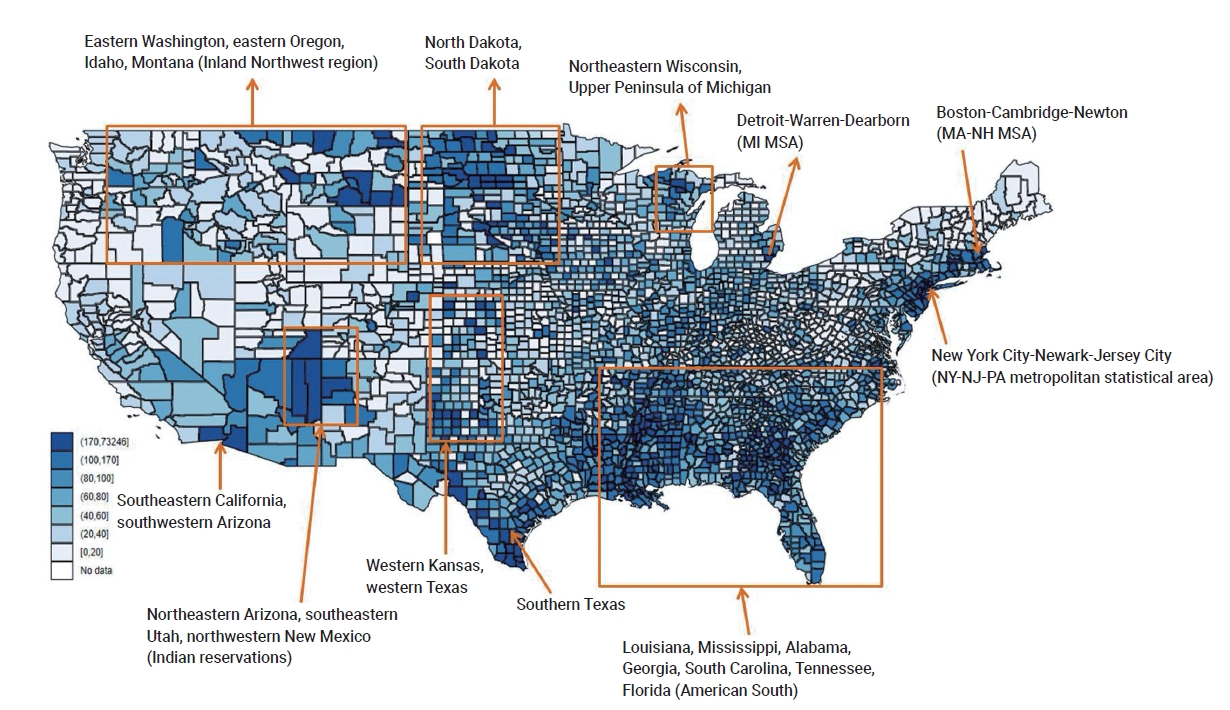
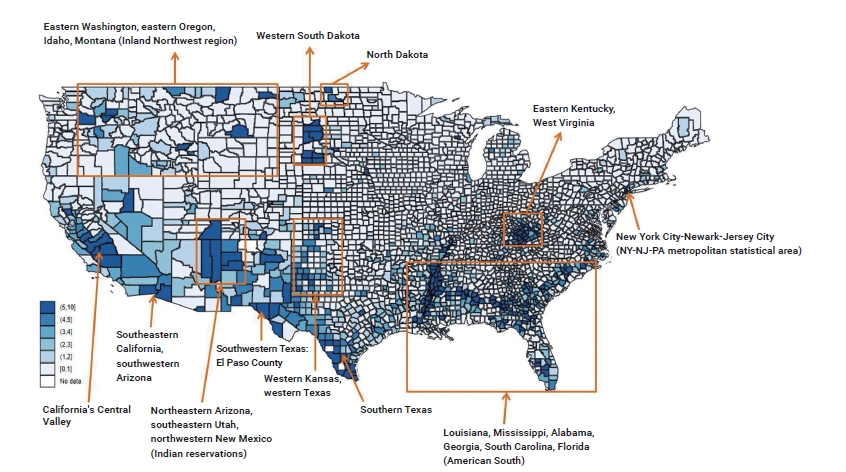
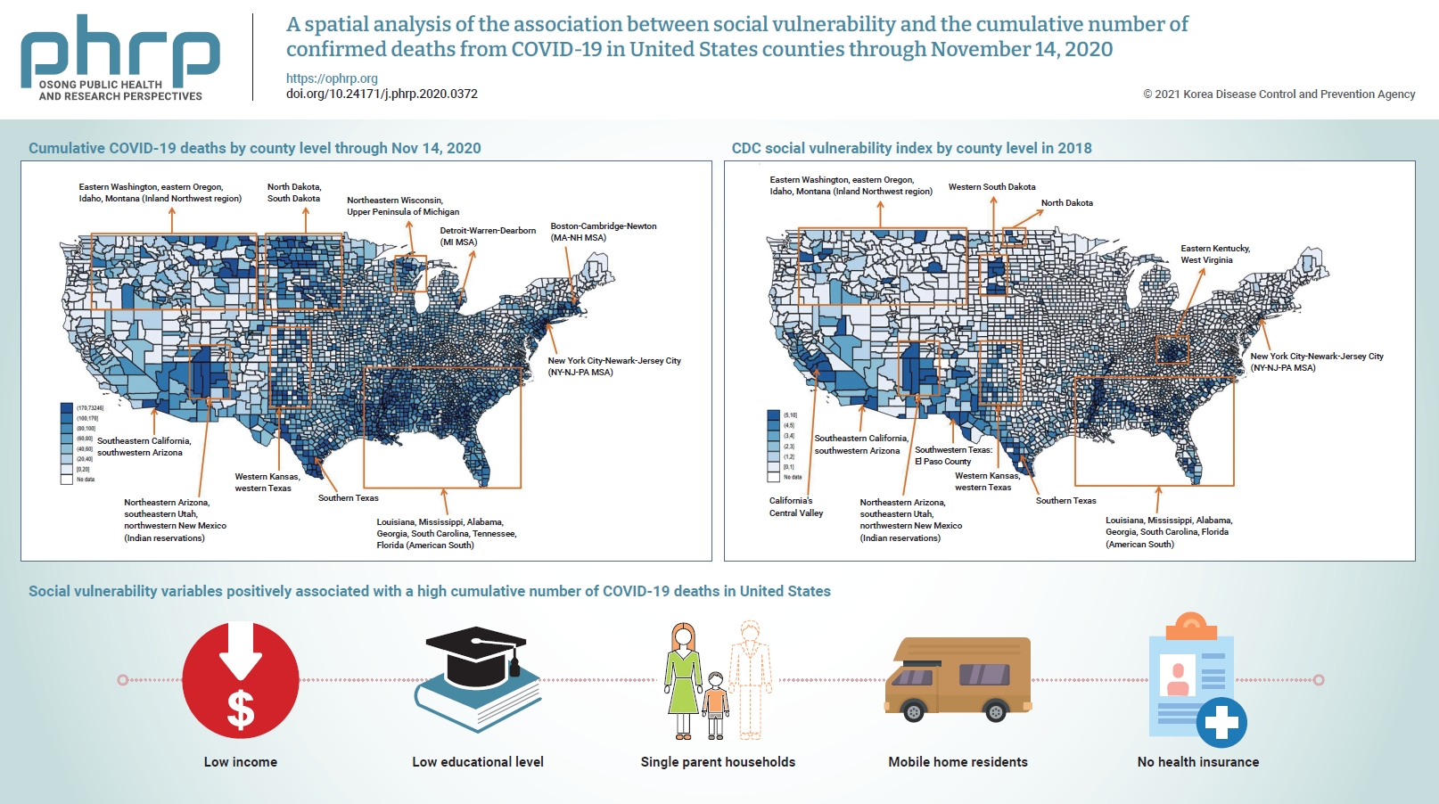
Table 1.Results from regression models
| Flags | Category | OLS (n=3,141) | Spatial lag (n=3,141) | Spatial error (n=3,141) |
|---|---|---|---|---|
| The percentage of persons in poverty is in the 90th percentile. | No | Ref | Ref | Ref |
| Yes | −0.007 (0.104) | 0.008 (0.096) | 0.051 (0.094) | |
| The percentage of civilian unemployment is in the 90th percentile. | No | Ref | Ref | Ref |
| Yes | 0.063 (0.085) | 0.049 (0.079) | 0.081 (0.078) | |
| Per capita income is in the 90th percentile. | No | Ref | Ref | Ref |
| Yes | 0.318** (0.102) | 0.216* (0.095) | 0.221* (0.093) | |
| The percentage of persons with no high school diploma is in the 90th percentile. | No | Ref | Ref | Ref |
| Yes | 0.370*** (0.093) | 0.280** (0.087) | 0.286** (0.089) | |
| The percentage of persons aged 65 and older is in the 90th percentile. | No | Ref | Ref | Ref |
| Yes | −0.324*** (0.079) | −0.254*** (0.073) | −0.285*** (0.076) | |
| The percentage of persons aged 17 and younger is in the 90th percentile. | No | Ref | Ref | Ref |
| Yes | −0.212* (0.085) | −0.170* (0.079) | −0.102 (0.083) | |
| The percentage of persons with a disability is in the 90th percentile. | No | Ref | Ref | Ref |
| Yes | −0.221** (0.080) | −0.172* (0.075) | −0.075 (0.080) | |
| The percentage of single parent households is in the 90th percentile. | No | Ref | Ref | Ref |
| Yes | 0.420*** (0.082) | 0.303*** (0.081) | 0.165* (0.082) | |
| The percentage of minorities is in the 90th percentile. | No | Ref | Ref | Ref |
| Yes | 0.117 (0.095) | 0.122 (0.088) | 0.052 (0.093) | |
| The percentage of those with limited English is in the 90th percentile. | No | Ref | Ref | Ref |
| Yes | 0.126 (0.091) | 0.116 (0.085) | 0.083 (0.088) | |
| The percentage of households in multi-unit housing complexes is in the 90th percentile. | No | Ref | Ref | Ref |
| Yes | −0.304*** (0.084) | −0.172* (0.078) | −0.350*** (0.079) | |
| The percentage of people living in mobile homes is in the 90th percentile. | No | Ref | Ref | Ref |
| Yes | 0.420*** (0.082) | 0.266** (0.077) | 0.302*** (0.081) | |
| The percentage of crowded households is in the 90th percentile. | No | Ref | Ref | Ref |
| Yes | −0.253** (0.092) | −0.134 (0.086) | −0.115 (0.087) | |
| The percentage of households with no vehicles is in the 90th percentile. | No | Ref | Ref | Ref |
| Yes | −0.017 (0.086) | 0.047 (0.080) | 0.059 (0.081) | |
| The percentage of persons in institutionalized group quarters is in the 90th percentile. | No | Ref | Ref | Ref |
| Yes | 0.161 (0.089) | 0.137 (0.083) | 0.069 (0.081) | |
| % of people with no health insurance | 0.041*** (0.005) | 0.032*** (0.005) | 0.034*** (0.006) | |
| Population (log-transformed) | 0.263*** (0.018) | 0.198*** (0.017) | 0.291*** (0.021) | |
| % of males | −0.060*** (0.010) | −0.045*** (0.011) | −0.031** (0.011) | |
| Constant | 3.473*** (0.651) | 2.274*** (0.608) | 1.751** (0.621) | |
| ρWY | - | 0.372*** (0.018) | - | |
| λWε | - | - | 0.561*** (0.024) | |
| −2logL | - | 9,764.87 | 9,712.02 | |
| Akaike information criterion | 10,179.03 | 9,806.87 | 9,754.02 |
Table 2.Descriptive statistics of other variables (n=3,141)
Table 3.Descriptive statistics of fifteen high social vulnerability variables (flags) (n=3,141)
| Flags | n | Mean±SDa) |
|---|---|---|
| The percentage of persons in poverty is in the 90th percentile. | ||
| No | 2,830 | 3.547±1.338 |
| Yes | 311 | 4.292±1.236 |
| The percentage of civilian unemployment is in the 90th percentile. | ||
| No | 2,829 | 3.574±1.338 |
| Yes | 312 | 4.045±1.236 |
| Per capita income is in the 90th percentile. | ||
| No | 2,826 | 3.551±1.330 |
| Yes | 315 | 4.248±1.336 |
| The percentage of persons with no high school diploma is in the 90th percentile. | ||
| No | 2,830 | 3.549±1.346 |
| Yes | 311 | 4.279±1.163 |
| The percentage of persons aged 65 and older is in the 90th percentile. | ||
| No | 2,837 | 3.697±1.256 |
| Yes | 304 | 2.917±1.861 |
| The percentage of persons aged 17 and younger is in the 90th percentile. | ||
| No | 2,828 | 3.600±1.342 |
| Yes | 313 | 3.810±1.379 |
| The percentage of persons with a disability is in the 90th percentile. | ||
| No | 2,830 | 3.638±1.322 |
| Yes | 311 | 3.467±1.550 |
| The percentage of single parent households is in the 90th percentile. | ||
| No | 2,832 | 3.532±1.339 |
| Yes | 309 | 4.437±1.121 |
| The percentage of minorities is in the 90th percentile. | ||
| No | 2,829 | 3.543±1.332 |
| Yes | 312 | 4.329±1.271 |
| The percentage of those with limited English is in the 90th percentile. | ||
| No | 2,826 | 3.568±1.358 |
| Yes | 315 | 4.094±1.139 |
| The percentage of households in multi-unit housing complexes is in the 90th percentile. | ||
| No | 2,826 | 3.599±1.380 |
| Yes | 315 | 3.823±0.975 |
| The percentage of people living in mobile homes is in the 90th percentile. | ||
| No | 2,829 | 3.560±1.342 |
| Yes | 312 | 4.172±1.258 |
| The percentage of crowded households is in the 90th percentile. | ||
| No | 2,839 | 3.591±1.336 |
| Yes | 302 | 3.907±1.409 |
| The percentage of households with no vehicles is in the 90th percentile. | ||
| No | 2,833 | 3.568±1.327 |
| Yes | 308 | 4.111±1.423 |
| The percentage of persons in institutionalized group quarters is in the 90th percentile. | ||
| No | 2,828 | 3.616±1.333 |
| Yes | 313 | 3.665±1.467 |
- 1. Centers for Disease Control and Prevention (CDC). Coronavirus disease 2019 (COVID-19) 2020 interim case definition, approved August 5, 2020 [Internet]. Atlanta: CDC; 2020 [cited 2020 Nov 18]. Available from: https://wwwn.cdc.gov/nndss/conditions/coronavirus-disease-2019-covid-19/case-definition/2020/08/05/.
- 2. USA Facts. US coronavirus cases and deaths. Track COVID-19 data daily by state and county [Internet]. USA Facts; 2020 [cited 2020 Nov 18]. Available from: https://usafacts.org/visualizations/coronavirus-covid-19-spread-map/.
- 3. Our World in Data. Statistics and research: mortality risk of COVID-19 [Internet]. Our World in Data; 2020 [cited 2020 Nov 18]. Available from: https://ourworldindata.org/mortality-risk-covid.
- 4. Centers for Disease Control and Prevention (CDC). estimated influenza illnesses, medical visits, hospitalizations, and deaths in the United States: 2018–2019 influenza season [Internet]. Atlanta: CDC; 2020 [cited 2020 Nov 18]. Available from: https://www.cdc.gov/flu/about/burden/2018-2019.html.
- 5. Blaikie P, Cannon T, Davis T, et al. At risk: natural hazards, people’s vulnerability and disasters. London: Routledge; 1994.
- 6. Hewitt K. Regions of risk: a geographical introduction to disasters. London: Routledge; 1997.
- 7. Wisner B, Blaikie P, Cannon T, et al. At risk: natural hazards, people’s vulnerability and disasters. 2nd ed. London: Routledge; 2004.
- 8. Kim SJ, Bostwick W. Social vulnerability and racial inequality in COVID-19 deaths in Chicago. Health Educ Behav 2020;47:509−13.ArticlePubMedPMC
- 9. Cutter SL, Finch C. Temporal and spatial changes in social vulnerability to natural hazards. Proc Natl Acad Sci U S A 2008;105:2301−6.ArticlePubMedPMC
- 10. Holand IS, Lujala P. Replicating and adapting an index of social vulnerability to a new context: a comparison study for Norway. Prof Geogr 2013;65:312−28.Article
- 11. Lixin Y, Xi Z, Lingling G, et al. Analysis of social vulnerability to hazards in China. Environ Earth Sci 2014;71:3109−17.Article
- 12. Chakraborty J, Tobin GA, Montz BE. Population evacuation: assessing spatial variability in geophysical risk and social vulnerability to natural hazards. Nat Hazards Rev 2005;6:23−33.Article
- 13. Flanagan BE, Gregory EW, Hallisey EJ, et al. A social vulnerability index for disaster management. J Homel Secur Emerg Manag 2011;8:3. Article
- 14. Martins VN, e Silva DS, Cabral P. Social vulnerability assessment to seismic risk using multicriteria analysis: the case study of Vila Franca do Campo (São Miguel Island, Azores, Portugal). Nat Hazards 2012;62:385−404.Article
- 15. Chen W, Cutter SL, Emrich CT, et al. Measuring social vulnerability to natural hazards in the Yangtze River Delta region, China. Int J Disaster Risk Sci 2013;4:169−81.Article
- 16. Emrich CT, Cutter SL. Social vulnerability to climate-sensitive hazards in the southern United States. Weather Clim Soc 2011;3:193−208.Article
- 17. Li F, Bi J, Huang L, et al. Mapping human vulnerability to chemical accidents in the vicinity of chemical industry parks. J Hazard Mater 2010;179:500−6.ArticlePubMed
- 18. Wood NJ, Burton CG, Cutter SL. Community variations in social vulnerability to Cascadia-related tsunamis in the U.S. Pacific Northwest. Nat Hazards 2010;52:369−89.Article
- 19. Arms I, Gavris A. Social vulnerability assessment using spatial multi-criteria analysis (SEVI model) and the Social Vulnerability Index (SoVI model): a case study for Bucharest, Romania. Nat Hazards Earth Syst Sci 2013;13:1481−99.Article
- 20. Schmidtlein MC, Deutsch RC, Piegorsch WW, et al. A sensitivity analysis of the social vulnerability index. Risk Anal 2008;28:1099−114.ArticlePubMed
- 21. Holand IS, Lujala P, Rod JK. Social vulnerability assessment for Norway: a quantitative approach. Nor Geogr Tidsskr 2011;65:1−17.Article
- 22. Morrow BH. Identifying and mapping community vulnerability. Disasters 1999;23:1−18.ArticlePubMed
- 23. Ge Y, Dou W, Gu Z, et al. Assessment of social vulnerability to natural hazards in the Yangtze River Delta, China. Stoch Environ Res Risk Assess 2013;27:1899−908.Article
- 24. Wallace LM, Theou O, Pena F, et al. Social vulnerability as a predictor of mortality and disability: cross-country differences in the survey of health, aging, and retirement in Europe (SHARE). Aging Clin Exp Res 2015;27:365−72.ArticlePubMed
- 25. de Oliveira Mendes JM. Social vulnerability indexes as planning tools: beyond the preparedness paradigm. J Risk Res 2009;12:43−58.Article
- 26. Fordham M, Lovekamp WE, Thomas DS, et al. In: Thomas DS, Phillips BD, Lovekamp WE, et al, editors. Social vulnerability to disasters. 2nd ed. Boca Raton, FL: CRC Press; 2013. p. 1-32.
- 27. Seddighi H. COVID-19 as a natural disaster: focusing on exposure and vulnerability for response. Disaster Med Public Health Prep 2020;14:e42−3.Article
- 28. Agency for Toxic Substances and Disease Registry (ATSDR). CDC Social Vulnerability Index (SVI): CDC SVI data and documentation download [Internet]. ATSDR; 2020 [cited 2020 Nov 18]. Available from: https://www.atsdr.cdc.gov/placeandhealth/svi/data_documentation_download.html.
- 29. United States Census Bureau. American Community Survey: 2014−2018 ACS 5-year data profile [Internet]. Washington, DC: United States Census Bureau; 2020 [cited 2020 Nov 18]. Available from: https://www.census.gov/acs/www/data/data-tables-and-tools/data-profiles/.
- 30. Anselin L. Lagrange multiplier test diagnostics for spatial dependence and spatial heterogeneity. Geogr Anal 1988;20:1−17.Article
- 31. Conway D, Li CQ, Wolch J, et al. A spatial autocorrelation approach for examining the effects of urban greenspace on residential property values. J Real Estate Finan Econ 2010;41:150−69.Article
- 32. Liu D. Spatial Autoregression in Stata. Cross-sectional Spatial Autoregression: spregress [Internet]. College Station (TX): StataCorp.; 2020 [cited 2020 Nov 18]. Available from: https://www.stata.com/training/webinar_series/spatial-autoregressive-models/spatial/resource/spregress.html.
- 33. Anselin L, Bera AK, Florax R, et al. Simple diagnostic tests for spatial dependence. Reg Sci Urban Econ 1996;26:77−104.Article
- 34. Menchik PL. Economic status as a determinant of mortality among black and white older men: does poverty kill? Popul Stud 1993;47:427−36.Article
- 35. Smith KR, Zick CD. Linked lives, dependent demise? Survival analysis of husbands and wives. Demography 1994;31:81−93.ArticlePubMed
- 36. Hart CL, Smith GD, Blane D. Inequalities in mortality by social class measured at 3 stages of the lifecourse. Am J Public Health 1998;88:471−4.ArticlePubMedPMC
- 37. Mirowsky J, Ross CE, Reynolds J. Links between social status and health status. Edited by Bird CE, Conrad P, Fremont AM: Handbook of medical sociology. Upper Saddle River (NJ): Prentice Hall Publishing; 2000. pp 47−67.
- 38. Friis K, Lasgaard M, Rowlands G, et al. Health literacy mediates the relationship between educational attainment and health behavior: a Danish population-based study. J Health Commun 2016;21(sup2). 54−60.ArticlePubMed
- 39. Spencer N. Maternal education, lone parenthood, material hardship, maternal smoking, and longstanding respiratory problems in childhood: testing a hierarchical conceptual framework. J Epidemiol Community Health 2005;59:842−6.ArticlePubMedPMC
- 40. Scharte M, Bolte G; GME Study Group. Increased health risks of children with single mothers: the impact of socio-economic and environmental factors. Eur J Public Health 2013;23:469−75.ArticlePubMed
- 41. Cancian M, Danziger S. Changing poverty, changing policies. New York: Russell Sage Foundation; 2009.
- 42. Brooks MM, Mueller JT. Factors affecting mobile home prevalence in the United States: Poverty, natural amenities, and employment in natural resources. Popul Space Place 2020;26:e2311.Article
- 43. Institute of Medicine, Board on Health Care Services, Committee on the Consequences of Uninsurance. Care without coverage: too little, too late. Washington, DC: National Academies Press; 2002.
- 44. Wilper AP, Woolhandler S, Lasser KE, et al. Health insurance and mortality in US adults. Am J Public Health 2009;99:2289−95.ArticlePubMedPMC
- 45. United States Census Bureau. Health insurance coverage in the United States: 2018 [Internet]. Washington, DC: United States Census Bureau; 2019 [cited 2020 Nov 26]. Available from https://www.census.gov/library/publications/2019/demo/p60-267.html.
- 46. Heinrich CJ, Scholz JK. Making the work-based safety net work better: forward-looking policies to help low-income families. New York: Russell Sage Foundation; 2009.
References
Figure & Data
References
Citations
Citations to this article as recorded by 
- Ecological comparison of six countries in two waves of COVID-19
Meiheng Liu, Leiyu Shi, Manfei Yang, Jun Jiao, Junyan Yang, Mengyuan Ma, Wanzhen Xie, Gang Sun
Frontiers in Public Health.2024;[Epub] CrossRef - Social vulnerability and COVID-19 in Maringá, Brazil
Matheus Pereira Libório, Oseias da Silva Martinuci, Patrícia Bernardes, Natália Cristina Alves Caetano Chav Krohling, Guilherme Castro, Henrique Leonardo Guerra, Eduardo Alcantara Ribeiro, Udelysses Janete Veltrini Fonzar, Ícaro da Costa Francisco
Spatial Information Research.2023; 31(1): 51. CrossRef - A county-level analysis of association between social vulnerability and COVID-19 cases in Khuzestan Province, Iran
Mahmoud Arvin, Shahram Bazrafkan, Parisa Beiki, Ayyoob Sharifi
International Journal of Disaster Risk Reduction.2023; 84: 103495. CrossRef - Global mapping of epidemic risk assessment toolkits: A scoping review for COVID-19 and future epidemics preparedness implications
Bach Xuan Tran, Long Hoang Nguyen, Linh Phuong Doan, Tham Thi Nguyen, Giang Thu Vu, Hoa Thi Do, Huong Thi Le, Carl A. Latkin, Cyrus S. H. Ho, Roger C. M. Ho, Md Nazirul Islam Sarker
PLOS ONE.2022; 17(9): e0272037. CrossRef - COVID-19 mortality and deprivation: pandemic, syndemic, and endemic health inequalities
Victoria J McGowan, Clare Bambra
The Lancet Public Health.2022; 7(11): e966. CrossRef
 PubReader
 ePub Link
 Cite
Cite


