Optimal Implementation of Intervention to Control the Self-harm Epidemic

Byul Nim Kim; M.A. Masud; Yongkuk Kim

doi:10.1016/j.phrp.2014.10.001

Articles

Page Path: HOME > Osong Public Health Res Perspect > Volume 5(6); 2014 > Article

Original Article Optimal Implementation of Intervention to Control the Self-harm Epidemic: Byul Nim Kim, M.A. Masud, Yongkuk Kim; Osong Public Health and Research Perspectives 2014;5(6):315-323.
DOI: https://doi.org/10.1016/j.phrp.2014.10.001
Published online: November 12, 2014

Department of Mathematics, Kyungpook National University, Daegu, Korea

∗Corresponding author. yongkuk@knu.ac.kr

• Received: August 3, 2014 • Revised: September 15, 2014 • Accepted: September 22, 2014

This is an Open Access article distributed under the terms of the CC-BY-NC License (http://creativecommons.org/licenses/by-nc/3.0).

3,353 Views
20 Download
3 Crossref
4 Scopus

prev next

Full Article

Download PDF

Abstract
Introduction
Materials and methods
Results
Discussion
Conflicts of interest
Acknowledgements
Article information
References

Abstract

Objectives
Deliberate self-harm (DSH) of a young person has been a matter of growing concern to parents and policymakers. Prevention and early eradication are the main interventional techniques among which prevention through reducing peer pressure has a major role in reducing the DSH epidemic. Our aim is to develop an optimal control strategy for minimizing the DSH epidemic and to assess the efficacy of the controls.
Methods
We considered a deterministic compartmental model of the DSH epidemic and two interventional techniques as the control measures. Pontryagin's Maximum Principle was used to mathematically derive the optimal controls. We also simulated the model using the forward-backward sweep method.
Results
Simulation results showed that the controls needed to be used simultaneously to reduce DSH successfully. An optimal control strategy should be adopted, depending on implementation costs for the controls.
Conclusion
The long-term success of the optimum control depends on the implementation cost. If the cost is very high, the control could be used for a short term, even though it fails in the long run. The control strategy, most importantly, should be implemented as early as possible to attack a comparatively fewer number of addicted individuals.
Keywords:
Keywords
contagious social issue; deliberate self-harm; epidemiological model; optimal control; Pontryagin's Maximal Principle

Introduction

Deliberate self-harm (DSH) is an activity of an individual in which the sole intention is to cause self-harm, although not to commit suicide; however, sometimes acute medical situations arise [1]. More scientific definitions of DSH are available in the literature [2–4]. It is associated with the physiology and psychology of the affected individual. In the past decade, it has become a pronounced health concern among adolescents and young adults all over the world [5]. You et al [6] and Whitlock [7] addressed it as a contagious social issue. Deliberate self-harm is associated with depression, anxiety, poor school performance, family conflict [8], sexual abuse [9], and other factors. Mathematical modeling of epidemics is a constructive tool to assess the evolution of contagious problems and to discover strategies to reduce or eradicate the epidemic of contagious problems.

The techniques of mathematical modeling have recently been utilized in problems related to human behaviors and social interaction. For example, the theory for social behavior of individuals subjected to the social interaction was developed by Wirl and Feichtinger [10] to address the problem of obesity. Mathematical models have also been used to study the obesity epidemic [11–16]. Such ideas are also used to study smoking dynamics mathematically [17–22]. In addition, Li [23] used Bayesian proportional hazard analysis to deal with school drop-out. Porco et al [24] presented two models for antibiotic abuse. The techniques of mathematical modeling are likewise being exercised to understand contagious social and behavioral epidemics from diverse viewpoints.

Do and Lee [25] proposed a mathematical model for the self-harm epidemic and analyzed it mathematically. By considering self-harm as a contagious disease, they formulated a deterministic compartmental model. In the present study, we introduced time-dependent controls into the Do and Lee model [25], and extend an optimal control problem to understand cost-effective strategies for reducing DSH.

2.1 Basic model: The Lee and Do model [25] without a demographic effect reduces to the following formula:

(1)
dSdt=−αSA+PNdAdt=αSA+PN+ωP−βAN(P+R)−θA−ηAdPdt=βAN(P+R)+θA−ρP−ωPdRdt=ηA+ρP; In this paper, we note that the whole population N(t) = S(t)+A(t)+P(t)+R(t) is constant. The variable N(t) includes only adolescents and young adults between the ages 12 years and 23 years and is divided into four classes: susceptible, S(t); addicted, A(t); in treatment P(t); and recovered, R(t). Individuals of S(t) who try DSH move to A(t) with the per capita transition rate, α, which is peer pressure on susceptible individuals in A(t) and P(t). Individuals repeating DSH remain in A(t), but individuals who stop DSH move to R(t) at the rate η. This is the rate at which individuals in A(t) stop DSH without any treatment program or individuals who tried DSH only once and transferred to R(t). When individuals in A(t) seek treatment, they go to P(t) at the rate of β(P+R)/N+θ. In this equation, β is peer pressure due to individuals in P(t) and R(t) to the individuals in A(t), and θ is the intervention rate at which addicted individuals seek treatment. If the treatment fails, individuals may go back to A(t) from P(t) at the rate ω. Individuals in P(t) recover at rate ρ and move to R(t). The values of α and β may be different, but in this study they are considered the same for homogeneous mixing. Among all of these parameters, the system is most sensitive to α and η [19]. The values of η may also increase or decrease, depending on the positive or negative influence of the Internet [26]. Furthermore, the individual who performs DSH once, seeks more serious injury for the next DSH episode [27]. Therefore, a control strategy should be concerned with prevention through controlling peer pressure α and early intervention η.
2.2 Optimal control: To shrink the DSH epidemic, we adopted two control strategies with the intent of increasing prevention [i.e., decreasing α and increasing early intervention (η)]. However, maintaining constant control over time is impractical. Therefore, our aim is to show that it is possible to implement time-dependent control techniques while minimizing the addicted population with minimum cost of implementation of the control measures.; To develop an optimal control problem for the aforementioned purpose, two control terms were introduced into the basic model (1). The model reduces to the following formula:

(2)
dSdt=−α(1−u1(t))SA+PNdAdt=α(1−u1(t))SA+PN+ωP−βAN(P+R)−θA−(η+μu2(t))AdPdt=βAN(P+R)+θA−ρP−ωPdRdt=(η+μu2(t))A+ρP; In this equation N = S(t)+A(t)+P(t)+R(t) is constant.; The control variables, u₁(t) and u₂(t), represent the quantity of intervention associated with the parameters α and η, respectively at time t. The factor of 1−u₁(t) reduces the per capita transition rate α from S(t) to A(t). The per capita transition rate η from P to R increases at a rate that is proportional to u₂(t) in which μ > 0 is the proportionality constant.; We define our control set as follows:
U:={(u1(t),u2(t)):u1(t)andu2(t)isLebesguemeasurableon[0,T];0≤u1(t),u2(t)≤1}; An optimal control problem with the objective cost functional can be given by

(3)
J(u1,u2)=∫0T(AcA(t)+B12u12(t)+B22u22(t))dt,0≤u1(t),u2(t)≤1
which is subject to the state equation (2). In the objective cost functional, the quantities A_c, B₁ and B₂ represent the weight constants. The costs associated with the controls of the transition rates are described by the terms B1u12(t) and B2u22(t). The variable A_c represents the degree of negative influence on the society by each addicted individual. The goal is to minimize the population A(t) of addicted individuals and the implementation cost of the controls. Therefore, we looked for optimal control functions (u1∗,u2∗) so that:

(4)
J(u1∗,u2∗)=min{J(u1,u2):(u1,u2)∈U},
which is subject to the system (2). To approach an optimal solution, we first defined the Hamiltonian function H for problems (2) and (3), and then used Pontryagin's Maximum Principle [28] to derive the characterization for the optimal control. The principle converts problems (2) and (3) into a problem of minimizing pointwise a Hamiltonian, H, with respect to u₁ and u₂. The integrand of the objective functional along with the four right hand sides of the state equations constitutes the Hamiltonian for our problem. So the Hamiltonian is given by,

(5)
H(X(t),u(t),Λ(t))=AcA(t)+B12u12(t)+B22u22(t)+Λ(t)(dX(t)dt)T,
in which X(t) = (S(t), A(t), P(t), R(t)), u(t) = (u₁(t), u₂(t)) and Λ(t) = (λ₁(t), λ₂(t), λ₃(t), λ₄(t)).; Therefore, H(X(t),u(t),Λ(t)) becomes:

(6)
H(X(t),u(t),Λ(t))=AcA(t)+B12u12(t)+B22u22(t)+λ1(t)(−α(1−u1(t))S(t)A(t)+P(t)N)+λ2(t)(α(1−u1(t))S(t)A(t)+P(t)N+ωP(t)−βA(t)N(P(t)+R(t))−θA(t)−(η+μu2(t))A(t))+λ3(t)(βA(t)N(P(t)+R(t))+θA(t)−ρP(t)−ωP(t))+λ4(t)((η+μu2(t))A(t)+ρP(t))
.; Let S^∗(t), A^∗(t), P^∗(t), R^∗(t) be optimal state solutions with associated optimal control variables u1∗(t) and u2∗(t) for the optimal control problems (2) and (3). Adjoint variables λ₁(t), λ₂(t), λ₃(t), λ₄(t) would then exist that satisfy
λ1′(t)=(λ1(t)−λ2(t))α(1−u1∗(t))A∗(t)+P∗(t)Nλ2′(t)=−Ac+(λ1(t)−λ2(t))α(1−u1∗(t))S∗(t)N∗+(λ2(t)−λ3(t))(βP∗(t)+R∗(t)N∗+θ)+(λ2(t)−λ4(t))(η+μu2∗(t))λ3′(t)=(λ1(t)−λ2(t))α(1−u1∗(t))S∗(t)N∗+(λ2(t)−λ3(t))(βA∗(t)N∗−ω)+(λ3(t)−λ4(t))ρλ4′(t)=(λ2(t)−λ3(t))βA∗(t)N∗
with the transversality condition (or the boundary condition)

(7)
λj(T)=0,j=1,2,3,4.; Furthermore, the optimal controls u1∗(t) and u2∗(t) are given by

(8)
u1∗(t)=min{1,max{0,1B1(αS∗(A∗+P∗)(λ2−λ1)N)}}u2∗(t)=min{1,max{0,μA∗(λ2−λ4)B2}}; (Please refer to Appendix 1 for the formulation in detail.)

Results

To find the optimal control strategy for controlling the self-harm epidemic of adolescents and young adults in institutional settings, an optimal control problem has been established, based on the model proposed by Do and Lee [25]. The optimal control problem consists of eight ordinary differential equations describing states and adjoint variables with two control variables. The state variables are “susceptible”, S; “addicted”, A; “in treatment”, P; and “recovered”, R; the control u₁ is associated with reducing peer pressure and the control u₂ is associated with early intervention. As a general shortcoming, full efficiency of the controls is unfeasible. To choose an upper bound for the controls, we considered the study of Dunlop et al [29] in which they found that 79% of young people learned about suicide from the newspaper or from friends and family, and 59% of them learned from an online source. We assumed the upper bound of each of the controls was 0.6. The rate constant μ is chosen to be 0.01 in accordance with the value of η. Using the parameter values summarized in Table 1, the problem is solved numerically by the forward-backward sweep method [30], along with the fourth order Runge-Kutta algorithm, which is subject to a wide range of plausible values of weight factors A_c, B₁ and B₂ because the weights should vary from group to group. For an institutional setting, we considered that the total population is N(0) = 10000 with S(0) = 8700, A(0) = 900, P(0) = 100, R(0) = 300. Time span for the simulation is [0, T], in which T = 60 months (i.e., 5 years).

Figure 1 depicts the dynamics of states with and without the controls when the weight factors are A_c = 1, B₁ = 500, B₂ = 500. The rightmost graphs in Figure 1 show the time-dependent control strategy in which we see that the controls u₁ and u₂ should be implemented at maximum for a long period and then gradually decreased to zero. The controls work fairly well for reducing the number of addicted population.

Let t₁ and t₂ be the period of time for maximum implementation of the optimal controls u₁ and u₂, respectively. The time t₁ and t₂ may depend on the weights A_c, B₁, B₂ and the initial conditions as well. Figure 2 depicts the changes of t₁ and t₂ with B₁ = 100–1000 and A_c = 1–100 while keeping B₂ = 200 fixed. Figure 2A shows that for A_c > 60, the time t₁ is the same for all B₁; however, for smaller A_c; the effect of B₁ to the change of t₁ is more pronounced. A smaller B₁ results in a higher t₁ and vice versa. Figure 2B shows that t₂ increases with A_c but it is not affected by B₁. Figure 3 depicts the changes of t₁ and t₂ with B₂ = 100–1000 and A_c = 1–100 while keeping B₁ = 200 fixed. The change of weight B₂ does not affect the change of t₁ for all A_c and also does not affect the change of t₂ for A_c > 40. Figure 4 depicts the changes of t₁ and t₂ with B₁ = 100–1000 and B₂ = 100–1000 while keeping A_c = 1 fixed. Figure 4A illustrates that changes in B₁ and B₂ negatively affect changes in t₁ and t₂, as we have already seen in Figures 2 and 3. In addition, for B₁ > 100 t₁ increases with B₂. However, B₁ has no noticeable effect in the change of t₂. Figure 5 depicts the changes of t₁ and t₂ with B₁ = 100–1000 and B₂ = 100–1000 while keeping A_c = 10 fixed. In this case, B₁, and B₂ have no effect on changes in t₂ and t₁, respectively.

The optimal control aims at reducing the number of addicted individuals while ensuring the least implementation cost of the two controls mentioned previously. Let Awith_controlB1,B2t and Awithout_controlB1,B2t be the number of addicted people with and without optimal control, respectively, for specific values of the parameters at time t∈[0,T], and define ΔAB1,B2t:=Awithout_controlB1,B2t−Awith_controlB1,B2t as the number of reductions in the addicted population because of optimal control. From the previous results, it is clear that higher values of B₁ and B₂ reduce the implementation of the controls and consequently ΔAB1,B2t. For successful implementation of the controls, the condition ΔAB1,B2t>0 is needed for all t∈[0,T]. However, Figure 6A shows that ΔAB1,B2T<0 for some combinations of B₁, B₂ which include higher values for both. Figure 6B shows the same phenomena for different initial conditions S(0) = 7400, A(0) = 1800, P(0) = 200, R(0) = 600. In this case ΔAB1,B2T<0 for comparatively lower and more values of B₁, B₂.

Discussion

An optimal control problem has been established that takes into consideration self-harm as a contagious disease. We considered two control strategies: (1) reducing peer pressure and (2) accelerating early intervention with their associated costs (i.e., B₁ and B₂, respectively). The control problem is solved using Pontryagin's Maximum Principle. In this circumstance, the negative effect of an addicted individual is parameterized by A_c. The simultaneous use of both controls reduces the self-harm epidemic by increasing susceptible individuals and reducing the addicted individuals remarkably. But the costs associated with control strategies and the weight A_c may not be the same in all groups of young people. Depending on the groups, the costs and the weight may be varied so that different control strategies are needed. For a higher weight of addicted individuals, we used nearly the same control strategy for the groups, even with different control costs, which agrees with our intuition that a greater weight requires greater effort from the controls, irrespective of the control cost. However, if the weight is low, a great effort by the controls is no longer necessary. As a result, the strategy varies from group to group, depending on the control costs associated with the groups. Controls are implemented in smaller numbers in groups with a high control cost and vice versa.

In the case of low weight, the strategy for early intervention is not affected by the cost associated with reducing peer pressure. However, if the cost of reducing peer pressure is high in some groups, it affects the reduction of peer pressure. As a result, the number of addicted individuals increase, which requires more effort for early intervention, even though it is expensive. Furthermore, the control strategies have no interdependency, resulting from the associated costs.

The simulations presented above also shows that the control strategy is affected by the initial condition and the control costs. In groups with a high control cost, the control strategy is unsuitable for the long run. If the initial number of addicted people in a population is high, the control fails for lower costs of the controls. Therefore, even if the control costs are high, early implementation gives better results rather than waiting and allowing the number of addicted individuals to increase.

Therefore, we conclude that the simultaneous use of the controls gives the desired outcome. In groups in which associated costs are high, the controls may fail after a long period. What is most important is that the control strategy should be implemented as early as possible to attack a comparatively fewer number of addicted individuals. To make the model more realistic, further efforts should be focused on including age-dependent peer pressure [31], which remains for our future work.

Conflicts of interest

The authors declare no conflicts of interest.

Appendix 1

Theorem 1

Let S^∗(t), A^∗(t), P^∗(t), R^∗(t) be the optimal state solutions with associated optimal control variables u1∗(t) and u2∗(t) for the optimal control problems (2) and (3). There then exist the adjoint variables λ₁(t), λ₂(t), λ₃(t), λ₄(t) that satisfy:

(9)

λ1′(t)=(λ1(t)−λ2(t))α(1−u1∗(t))A∗(t)+P∗(t)Nλ2′(t)=−Ac+(λ1(t)−λ2(t))α(1−u1∗(t))S∗(t)N∗+(λ2(t)−λ3(t))(βP∗(t)+R∗(t)N∗+θ)+(λ2(t)−λ4(t))(η+μu2∗(t))λ3′(t)=(λ1(t)−λ2(t))α(1−u1∗(t))S∗(t)N∗+(λ2(t)−λ3(t))(βA∗(t)N∗−ω)+(λ3(t)−λ4(t))ρλ4′(t)=(λ2(t)−λ3(t))βA∗(t)N∗

with transversality condition (or boundary condition):

λj(T)=0,j=1,2,3,4.

Furthermore, the optimal controls u1∗(t) and u2∗(t) are given by:

(10)

u1∗(t)=min{1,max{0,1B1(αS∗(A∗+P∗)(λ2−λ1)N)}}u2∗(t)=min{1,max{0,μA∗(λ2−λ4)B2}}

Proof

To determine the adjoint equations and the transversality conditions, use the Hamiltonian (7). By Pontryagin's Maximum Principle, setting S(t) = S^∗(t), A(t) = A^∗(t), P(t) = P^∗(t), R(t) = R^∗(t) and differentiating the Hamiltonian (6) with respect to S(t), A(t), P(t), R(t), the following is obtained:

λ1′(t)=−∂H∂S=λ1(t)α(1−u1∗(t))A∗(t)+P∗(t)N(t)−λ2(t)α(1−u1∗(t))A∗(t)+P∗(t)N(t)λ2′(t)=−∂H∂A=−Ac+λ1(t)α(1−u1∗(t))S∗(t)N∗(t)−λ2(t)α(1−u1∗(t))S∗(t)N∗(t)+λ2(t)(βP∗(t)+R∗(t)N∗(t)+θ)+λ2(t)(η+μu2∗(t))−λ3(t)(βP∗(t)+R∗(t)N∗(t)+θ)−λ4(t)(η+μu2∗(t))λ3′(t)=−∂H∂P=λ1(t)α(1−u1∗(t))S∗(t)N∗(t)−λ2(t)α(1−u1∗(t))S∗(t)N∗(t)+λ2(t)βA∗(t)N∗(t)−λ2(t)ω−λ3(t)βA∗(t)N∗(t)+λ3(t)ω+λ3(t)ρ−λ4(t)ρλ4′(t)=−∂H∂H=λ2(t)βA∗(t)N∗(t)−λ3(t)βA∗(t)N∗(t)

which reduces to (9).

To obtain the optimality conditions (10), the Hamiltonian, H, is differentiated with respect to u₁(t), u₂(t). It is set equal to zero.

0=∂H∂u1=B1u1∗(t)+λ1(t)αS∗(t)A∗(t)+P∗(t)N(t)−λ2(t)αS∗(t)A∗(t)+P∗(t)N(t)0=∂H∂u2=B2u2∗(t)−λ2(t)μA∗(t)+λ4(t)μA∗(t)

Solving for the optimal controls obtains:

u1∗(t)=αS∗(t)(A∗(t)+P∗(t))(λ2(t)−λ1(t))B1Nu2∗(t)=μA∗(t)(λ2(t)−λ4(t))B2

To determine an explicit expression for the optimal controls for 0≤u1∗(t),u2∗(t)≤1, a standard optimality technique is utilized. We considered the following three cases.

On the set: {t:0<u1∗(t)<1}, ∂H∂u1=0. Hence, the optimal control is:

u1∗(t)=αS∗(t)(A∗(t)+P∗(t))(λ2(t)−λ1(t))B1N

In the set: {t:u1∗(t)=0}, ∂H∂u1≥0. This implies that:

λ1(t)αS∗(t)A∗(t)+P∗(t)N−λ2(t)αS∗(t)A∗(t)+P∗(t)N≥0

in which: αS∗(t)(A∗(t)+P∗(t))(λ2(t)−λ1(t))B1N≤0=u1∗(t)

In the set: {t:u1∗(t)=1}, ∂H∂u1≤0. This implies that:

λ1(t)αS∗(t)A∗(t)+P∗(t)N−λ2(t)αS∗(t)A∗(t)+P∗(t)N≤−B1

in which: αS∗(t)(A∗(t)+P∗(t))(λ2(t)−λ1(t))B1N≥1=u1∗(t)

Combining these three equations, results in the characterization of u1∗:

u1∗(t)=min{1,max{0,1B1(αS∗(A∗+P∗)(λ2−λ1)N)}}

Using similar arguments, a second optimal control function is obtained:

u2∗(t)=min{1,max{0,μA∗(λ2−λ4)B2}}.

Acknowledgements

Acknowledgements

This work was supported by Kyungpook National University Research Fund, (Daegu, Korea), 2012.

Article information

This is an Open Access article distributed under the terms of the Creative Commons Attribution Non-Commercial License (http://creativecommons.org/licenses/by-nc/3.0) which permits unrestricted non-commercial use, distribution, and reproduction in any medium, provided the original work is properly cited.

References

1. NHS Centre for Reviews and Dissemination . no. 6. Effective health care bulletin: deliberate self-harm. vol. 4:1998. University of York; York, United Kingdom.
2. Favazza A.. Why patients mutilate themselves. Hosp Community Psychiatry 40(2). 1989 Feb;137−145. Article PubMed
3. Madge N., Hewitt A., Hawton K.. Deliberate self-harm within an international community sample of young people: comparative findings from the Child and Adolescent Self-harm in Europe (CASE) Study. J Child Psychol Psychiatry 49(6). 2008 Jun;667−677. Article PubMed
4. Mangnall J., Yurkovich E.. A literature review of deliberate self-harm. Perspect Psychiatr Care 44(3). 2008 Jul;175−184. Article PubMed
5. Skegg K.. Self-harm. Lancet 366:2005 Oct;1471−1483. Article PubMed
6. You J., Lin M.P., Fu K.. The best friend and friendship group influence on adolescent nonsuicidal self-injury. J Abnorm Child Psychol 41(6). 2013 Aug;993−1004. Article PubMed
7. Whitlock J.. Self-Injurious behavior in adolescents. PLoS Medicine 7(5). 2010 May;e1000240Article PubMed
8. Laukkanen E., Rissanen M.-L., Honkalampi K.. The prevalence of self-cutting and other self-harm among 13- to 18-year-old Finnish adolescents. Soc Psychiatry Psychiatr Epidemiol 44(1). 2009 Jan;23−28. Article PubMed
9. Romans S.E., Martin J.L., Anderson J.C.. Sexual abuse in childhood and deliberate self-harm. Am J Psychiatry 152(9). 1995 Sep;1336−1342. Article PubMed
10. Wirl F., Feichtinger G.. Modelling social dynamics (of obesity) and thresholds. Games 1(4). 2010 Jul;395−414.Article
11. González-Parra G., Acedo L., Villanueva Micó R.-J., Arenas A.J.. Modeling the social obesity epidemic with stochastic networks. Physica A 389(17). 2010 Sep;3692−3701.Article
12. Jódar L., Santonja F.J., González-Parra G.. Modeling dynamics of infant obesity in the region of Valencia, Spain. Comput Math Appl 56(3). 2008 Aug;679−689.Article
13. Kim M.S., Chu C., Kim Y.. A Note on obesity as epidemic in Korea. Osong Public Health Res Perspect 2(2). 2011 Sep;135−140. Article PubMed
14. Santonja F.J., Villanueva R.J., Jódar L.. Mathematical modeling of social obesity epidemic in the region of Valencia, Spain. Mathematical and Computer Modeling of Dynamical Systems: Methods. Tools and Applications in Engineering and Related Sciences 16(1). 2010 Feb;23−34.
15. Santonja F.J., Shaikhet L.. Probabilistic stability analysis of social obesity epidemic by a delayed stochastic model. Nonlinear Analysis: Real World Applications 17:2014 Jun;114−125.Article
16. Aldila D., Rarasati N., Nuraini N.. Optimal control problem of treatment for obesity in a closed population. Int J Math Math Sci 2014:2014;Article ID 273037. http://dx.doi.org/10.1155/2014/273037.Article
17. Castillo-Garsow C., Jordan-Salivia G., Herrera A.R.. Mathematical models for the dynamics of tobacco use, recovery, and relapse. Technical Report Series BU-1505-M. 1997. Cornell University; Ithaca, NY.
18. Castillo G.C., Jordan S.G., Rodriguez A.H.. Mathematical models for the dynamics of tobacco use, recovery and relapse. Technical Report Series BU-1505-M. 2000. Cornell University Department of Biometrics; Ithaca, NY.
19. Sharomi O., Gumel A.B.. Curtailing smoking dynamics: a mathematical modeling approach. Appl Math Comput 195(2). 2008 Feb;475−499.Article
20. Lahrouz A., Omari L., Kiouach D.. Deterministic and stochastic stability of a mathematical model of smoking. Stat Probab Lett 81(8). 2011 Aug;1276−1284.Article
21. Alkhudhari Z., Al-Sheikh S., Al-Tuwairqi S.. Global dynamics of a mathematical model on smoking. ISRN Applied Mathematics 2014;Article ID 847075.Article
22. Timms K.P., Rivera D.E., Collins L.M.. Continuous-time system identification of a smoking cessation intervention. Int J Control 87(7). 2014 Feb;1423−1437. Article PubMed
23. Li M.. Bayesian proportional hazard analysis of the timing of high school dropout decisions. Econom Rev 26(5). 2007 Aug;529−556.Article
24. Porco T.C., Gao D., Scott J.C.. When does overuse of antibiotics become a tragedy of the commons? PLoS One 7(12). 2012;e46505Article PubMed PMC
25. Do T.S., Lee Y.S.. A modeling perspective of deliberate self-harm. Journal of KSIAM 14(4). 2010;275−284.
26. Daine K., Hawton K., Singaravelu V.. The power of the web: a systematic review of studies of the influence of the internet on self-harm and suicide in young people. PLoS One 8(10). 2013 Oct;e77555Article PubMed
27. Evans J., Reeves B., Platt H.. Impulsiveness, serotonin genes and repetition of deliberate self-harm (DSH). Psychol Med 30(6). 2000 Nov;1327−1334. Article PubMed
28. Agrachev A., Sachkov Y.. Control theory from the geometric viewpoint. 2004. Springer; Berlin, Germany.
29. Dunlop S.M., More E., Romer D.. Where do youth learn about suicides on the Internet, and what influence does this have on suicidal ideation? J Child Psychol Psychiatry 52(10). 2011 Oct;1073−1080. Article PubMed
30. Lenhart S., Workman J.T.. Optimal control applied to biological models. 2007. United Kingdom: Chapman and Hall/CRC; London: 책.
31. Moran P., Coffey C., Romaniuk H.. The natural history of self-harm from adolescence to young adulthood: a population-based cohort study. Lancet 379(9812). 2012 Jan;236−243. Article PubMed

Figure 1

The dynamics of states with and without controls when the weight factors are A_c = 1, B₁ = 500, B₂ = 500.

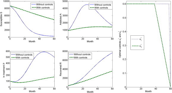
Figure 2

(A) The duration of maximum implementation for the optimal control u_1. In this equation, A_c = 1–100, B₁ = 100–1000, and B₂ = 200. (B) The duration of maximum implementation for the optimal control u_2. In this equation, A_c = 1–100, B₁ = 100–1000, and B₂ = 200.

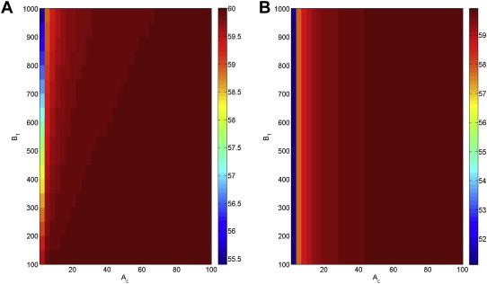
Figure 3

(A). The duration of maximum implementation for the optimal control U₁. In this equation, A_c = 1–100, B₂ = 100–1000, and B₁ = 200. (B). The duration of maximum implementation for the optimal control U₂. In this equation, A_c = 1–100, B₂ = 100–1000, and B₁ = 200.

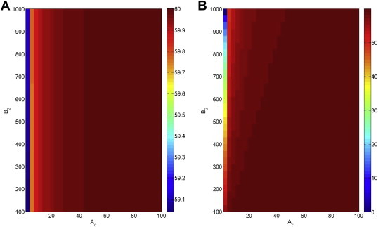
Figure 4

(A). The duration of maximum implementation for the optimal control U₁. In this equation, A_c = 1, B₁ = 100–1000, and B₂ = 100–1000. (B). The duration of maximum implementation for the optimal control U₂. In this equation, A_c = 1, B₁ = 100–1000, and B₂ = 100–1000.

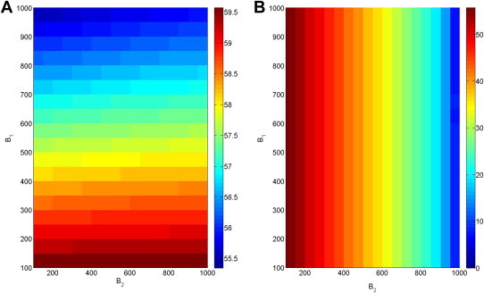
Figure 5

(A). The duration of the maximum implementation for the optimal control u1. In this equation, A_c = 10, B₁ = 100–1000, and B₂ = 100–1000. (B). The duration of the maximum implementation for the optimal control u2. In this equation, A_c = 10, B₁ = 100–1000, and B₂ = 100–1000.

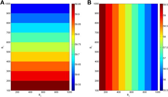
Figure 6

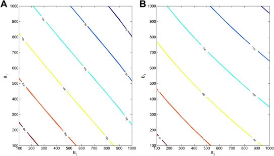
(A) The contour plot of ΔAB1,B2T for the initial conditionsS(0) = 8700, A(0) = 900, P(0) = 100, R(0) = 300. (B) The contour plot of ΔAB1,B2T for initial conditions S(0) = 7400, A(0) = 1800, P(0) = 200, R(0) = 600.

Table 1

The parameter values for the model.

Parameters	α	ω	β	θ	η	ρ	μ
Value (per mo.)	0.17	0.018	0.024	0.0042	0.03	0.08	0.01

^∗All values of the parameters are adopted from the results of parameter estimation in [25].

Figure & Data

References

Citations

Citations to this article as recorded by

A review of the use of optimal control in social models
D. M. G. Comissiong, J. Sooknanan
International Journal of Dynamics and Control.2018; 6(4): 1841. CrossRef
Adolescent self‐harm and risk factors
Jixiang Zhang, Jianwei Song, Jing Wang
Asia-Pacific Psychiatry.2016; 8(4): 287. CrossRef
Optimal Intervention Strategies for the Spread of Obesity
Chunyoung Oh, Masud M A
Journal of Applied Mathematics.2015; 2015: 1. CrossRef

PubReader
Cite

Cite

export Copy Format

Close

XML Download

Figure

Articles

Abstract

Keywords

Introduction

Materials and methods

(1)

(2)

(3)

(4)

(5)

(6)

(7)

(8)

Results

Discussion

Conflicts of interest

Theorem 1

(9)

(10)

Proof

Acknowledgements

Article information

References

Figure & Data

References

Citations

Figure 1

Figure 2

Figure 3

Figure 4

Figure 5

Figure 6

Table 1