
Articles
- Page Path
- HOME > Osong Public Health Res Perspect > Volume 3(3); 2012 > Article
-
Articles
Optimal Control Strategy ofPlasmodium vivax Malaria Transmission in Korea - Byul Nim Kima, Kyeongah Nahb, Chaeshin Chuc, Sang Uk Ryud, Yong Han Kange, Yongkuk Kima
-
Osong Public Health and Research Perspectives 2012;3(3):128-136.
DOI: https://doi.org/10.1016/j.phrp.2012.07.005
Published online: June 30, 2012
aDepartment of Mathematics, Kyungpook National University, Daegu, Korea.
bBolyai Institute, University of Szeged, Szeged, Hungary.
cDivision of Epidemic Intelligence Service, Korea Centers for Disease Control and Prevention, Osong, Korea.
dDepartment of Mathematics, Jeju National University, Jeju, Korea.
eInstitute of Liberal Education, Catholic University of Daegu, Daegu, Korea.
- Corresponding author. E-mail: yongkuk@knu.ac.kr
• Received: July 9, 2012 • Revised: July 15, 2012 • Accepted: July 20, 2012
Copyright ©2012, Korea Centers for Disease Control and Prevention
This is an Open Access article distributed under the terms of the Creative Commons Attribution Non-Commercial License () which permits unrestricted non-commercial use, distribution, and reproduction in any medium, provided the original work is properly cited.
Abstract
-
Objective
- To investigate the optimal control strategy for Plasmodium vivax malaria transmission in Korea.
-
Methods
- A Plasmodium vivax malaria transmission model with optimal control terms using a deterministic system of differential equations is presented, and analyzed mathematically and numerically.
-
Results
- If the cost of reducing the reproduction rate of the mosquito population is more than that of prevention measures to minimize mosquito-human contacts, the control of mosquito-human contacts needs to be taken for a longer time, comparing the other situations. More knowledge about the actual effectiveness and costs of control intervention measures would give more realistic control strategies.
-
Conclusion
- Mathematical model and numerical simulations suggest that the use of mosquito-reduction strategies is more effective than personal protection in some cases but not always.
- Malaria is a mosquito-borne infectious disease caused by a eukaryotic protist of the genus Plasmodium. Malaria is naturally transmitted by the bite of a female Anopheles mosquito. The primary vector in Korea is reported to be A sinensis. Since the re-emergence of Plasmodium vivax malaria in 1993[1,2], it has been endemic and continues to cause extensive morbidity in Korea, despite the huge efforts invested to control it.
- The first mathematical malaria model proposed by Ross [3], was subsequently modified by MacDonald, which has influenced both the modeling and the application of control strategies to malaria [4]. Recently, the optimal control theory has been applied to malaria Okosun et al [5], and to vector-borne disease Lashari
- The description of parameters for the model
- et al [6], who modified the model of Blayneh et al [7], but introduced some awkward terms.
- Models for Plasmodium flaciparum malaria or vector-borne diseases have been studied by many researchers [8-10]. In contrast, models for P vivax malaria are rare. Recently, Nah et al [11] proposed a model of P vivax malaria transmission. In this paper, by combining the ideas of Blayneh et al [7] and Nah et al [11], we propose the deterministic model of P vivax malaria transmission with optimal control terms. Using the optimal control theory, we sought optimal control strategies of P vivax malaria transmission in Korea.
1. Introduction
Table 1.
- 2.1. Model description: optimal control
- To construct a deterministic model for P vivax malaria transmission with control terms, the model of Nah et al [11] was modified and optimal control terms inspired by the model of Blayneh et al [7] were added as follows:
- In the model, human population H(t) is divided into four classes: susceptible (SH), short term exposed (EsH), long term exposed (ElH), and infectious (IH). Mosquito population M(t) is also divided into two classes: susceptible (SM), and infectious (IM). Note that the mosquito population M(t) is not constant while human population H(t) is constant.
- The factor of 1 – u1(t) reduces the reproduction rate of the mosquito population. It is assumed that the mortality rate of mosquitoes (susceptible and infected) increases at a rate proportional to u1(t), where ρ > 0 is a rate constant. In the human population, the associated force of infection is reduced by a factor of 1 – u2(t), where u2(t) measures the level of successful prevention efforts. In fact, the control u2(t) represents the use of prevention measures to minimize mosquito-human contacts. Table 1 lists detailed descriptions of the parameters. The system (1) has a unique solution set. (See Appendix A for detail.)
- An optimal control problem can now be formulated for the transmission dynamics of P vivax malaria transmission in Korea. The goal is to show that it is possible to implement time dependent anti-malaria control techniques while minimizing the cost of implementation of such control measures.
- The parameter values for the model
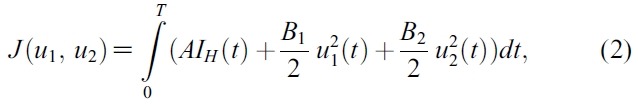
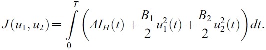
- An optimal control problem with the objective cost functional can be given by
- subject to the state system given by (1).
- The goal is to minimize the infected human populations and the cost of implementing the control. In the objective cost functional, the quantities A , B1 and B2 represent the weight constants of infected human, for mosquito control and prevention of mosquito-human contacts, respectively. The costs associated with mosquito control and prevention of mosquito-human contacts are described in the terms
- and
- respectively.
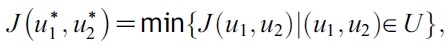
- Optimal control functions
- need to be found such that
- subject to the system of equations given by (1), where U = [(u1,u2)│ui(t) is piecewise continuous on [0, T], 0 ≤ui(t) ≤ 1, i = 1, 2} is the control set:
- Such optimal control functions
- exist, and the optimality system can be derived. (See Appendix B for detail.)
- 2.2. Numerical simulation
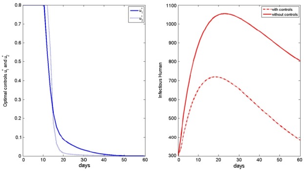
- Using the forward-backward sweep method, the optimality system was solved numerically. This consists of 12 ordinary differential equations from the state and adjoint equations, coupled with the two controls. In choosing upper bounds for the controls, it was supposed that the two controls would not be 100% effective, so the upper bounds of u1 and u2 were chosen to be 0.8. The weight in the objective functional is A1 = 1000. The parameters in Table 2 were adopted from other articles [11] and used for our simulation.
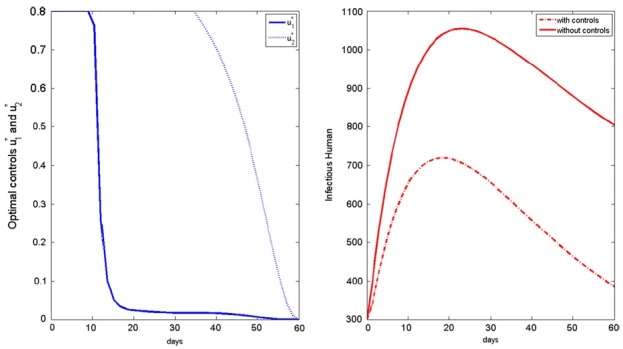
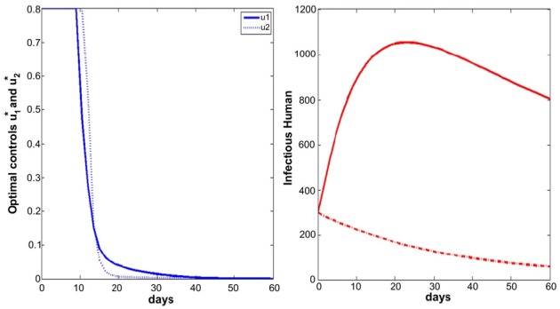
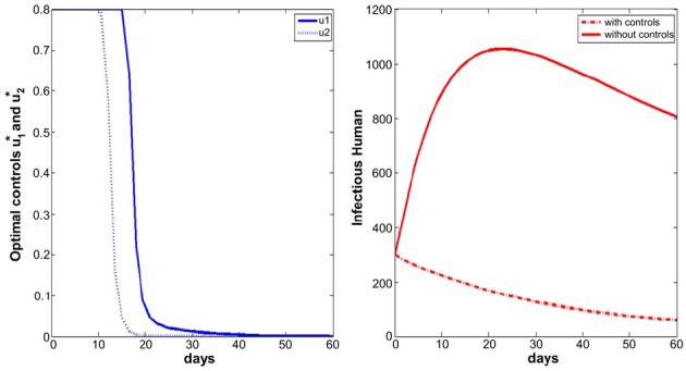
- We simulate the model in different scenarios. Figure 1 depicts scenarios for the state variables of the model for the case when the cost is the same for the two controls. Figure 2 depicts scenarios for the state variables of the model for the case when the cost of prevention measures to minimize mosquito-human contact is more expensive than the cost of reducing the reproduction rate of the mosquito population. Figure 3 depicts scenarios for the state variables of the model for the case when the cost of reducing the reproduction rate of the mosquito population are more expensive than the cost of prevention measures to minimize mosquito-human contacts.
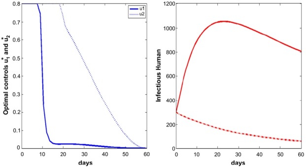
- It is also worth noting that different initial mosquitoes populations do not have effect on the optimal strategies (Figures 4 - 6).
- 2.3. Results
- If the cost of reducing the reproduction rate of the mosquito population is more than that of prevention measures to minimize mosquito-human contacts, the u2 control needs to be taken for a longer time, comparing the other situations (Figures 1 to 3). In that situation, full effort for u2 is needed after the high peak of infected human population.
- On the other hand, Figures 4 to 6 suggest that even though the mosquito population is not so high in initial point, full efforts for u1 and u2 are needed for at least some of the time.
2. Materials and Methods
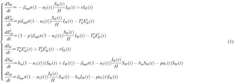
Table 2.
| Parameter | Value |
|---|---|
|
|
|
| bm | 0.7949 [0.1,1.5] |
| bmh | 0.5 |
| βhm | 0.5 |
| σ | 0.3 [0.25,0.5] |
| r | 0.07 [0.01,0.5] |
| p | 0.25 |
| Tsh | 1/25.9 |
| Tlh | 1/360.3 |


- After 1993’s reemergence of malaria, the endemicity of P vivax malaria is becoming a growing concern in South Korea. Public health advisories were subsequently issued to apply community mosquito control and personal protection.
- The purpose of this work is to suggest optimal control strategies of P vivax malaria in different scenarios. In all cases, optimal control programs lead effectively reduce the number of infectious individuals. We have used a deterministic model with time-dependent parameters to develop the transmission dynamics of P vivax malaria in Korea. For numerical simulations, most parameters were adopted from other articles [11].
- Mathematical model and numerical simulations suggest that the use of mosquito-reduction strategies is more effective than personal protection in some cases but not always. Public health authorities should choose the proper control strategy where their situation lies in the scenarios discussed in the Results section.
- Appendix A. The existence and uniqueness of solution
- We consider system (1). We obtain the existence and uniqueness of solution. In here we are given a suitable control set.
- Theorem 1. The system (1) with any initial condition has a unique solution.
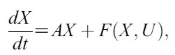
- Proof. We can rewrite (1) as :
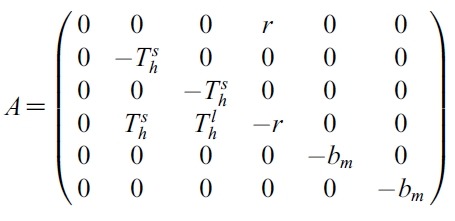
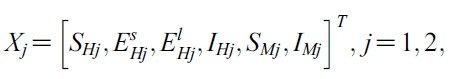
- where X = [SH, EsH, ElH, IH, SM, IM]T,
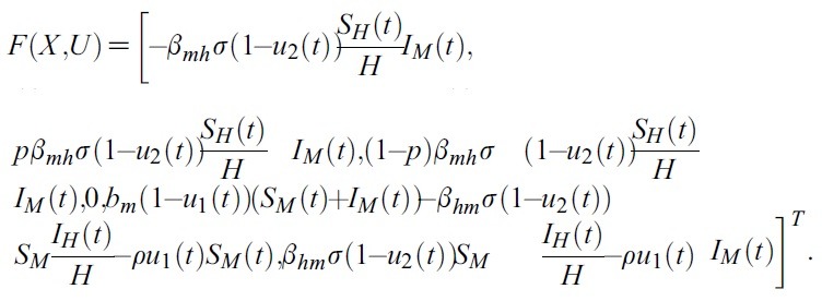
- U = [u1, u2]T and
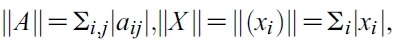
- So let G(X,U) = AX+F (X,U). Defined matrix A is a linear. So A is a bounded operator. Define a matrix norm and a vector norm as follows
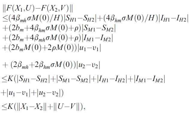
- respectively. To show the existence of solution of the system (1), we have to prove that F (X ,U). satisfy a Lipschitz condition. Let
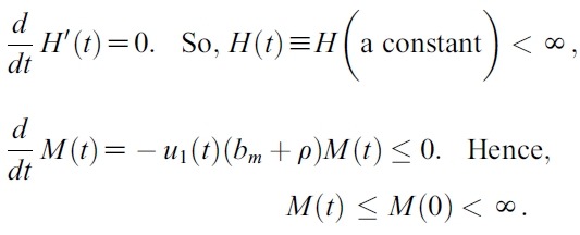
- H(t) : = SH(t)+EsH(t) + ElH(t)+IH(t).
- and
- M(t) : =SM(t) + IM (t)
- But
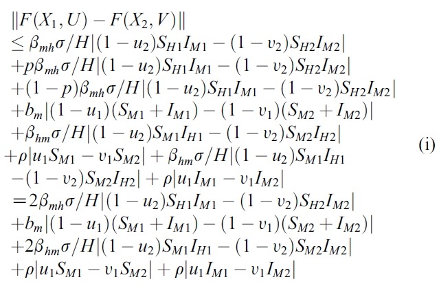
- For any given pairs (X1, U), (X2, V)
- U = (u1 , u2)T , V = (v1, v2)T, we obtain,
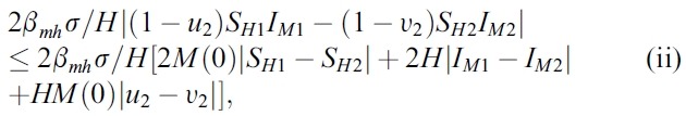
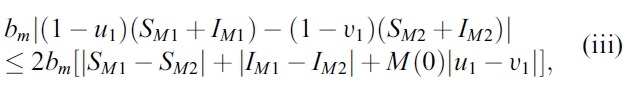
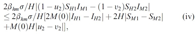
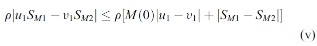
- We estimate the 4 terms in the right side of (i):
- and
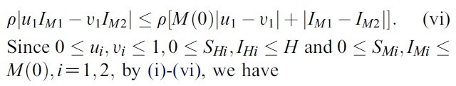
- where
- Hence, the system (1) satisfy all conditions of the Picard-Lindelof Theorem ([12,13]) and also the function F(X, U) is continuously differentiable. Therefore, the system (1) have a unique solution.
- Appendix B. Analysis of optimal control control problem
- We are to prove the existence of optimal control pairs for the system (1). Firstly, We set control space
- U = {(u1 , u2) │ui is piecewise continuous on [0, T],0 ≤ ui(t) ≤ 1, i = 1, 2}.
- We consider an optimal control problem to minimize the objective functional:
- Theorem 2. There exist an optimal control
- and
- such that
- subject to the control system (1) with initial conditions.- Proof. To prove the existence of an optimal control pairs we use the result in [14]. The set of control and corresponding state variables is a nonempty. Because for each control pairs we have proved in the Theorem 1 that there exists corresponding state solutions. And also it is ok when the control u1 = u2 = 0. Note that the control and the state variables are nonnegative values. The control space U is close and convex by definition. In the minimization problem, the convexity of the objective functional in u1 and u2 have to satisfy. The integrand in the functional,
- is convex function on the control u1 and u2. Also we can easily check that there exist a constant ρ > 1, a numbers ω1 ≥ 0 and ω2 > 0 such that
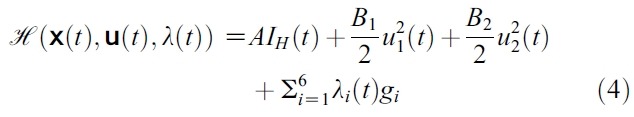
- which completes the existence of an optimal control.To find the optimal solution we apply Pontryagin’s Maximum Principle ([15-17]) to the constrained control problem, then the principle converts (1), (2) and (3) in to a problem of minimizing pointwise a Hamiltonian,
- with respect to u1 and u2. The Hamiltonian for our problem is the integrand of the objective functional coupled with the six right hand sides of the state equations:
- where gi is the right hand side of the differential equation of the ith state variable and also
- x(t) = (SH, EsH, ElH, IH, SM, IM), u(t) = (u1(t), u2(t)) and λ(t) = (λ1(t), λ2(t), (λ3(t), λ4(t), λ5(t), λ6(t)).
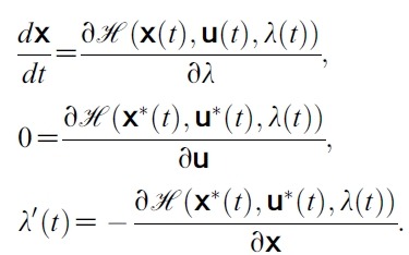
- By applying Pontryagin’s Maximum Principle([18]) if (x*(t), u*(t)) is an optimal control, then there exists a non-trivial vector function λ(t) satisfying the following equalities:
- If follows from the derivation above
- Now, we apply the necessary conditions to the Hamiltonian
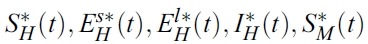
- Theorem 3. Let
- and
- be optimal state solutions with associated optimal control variables
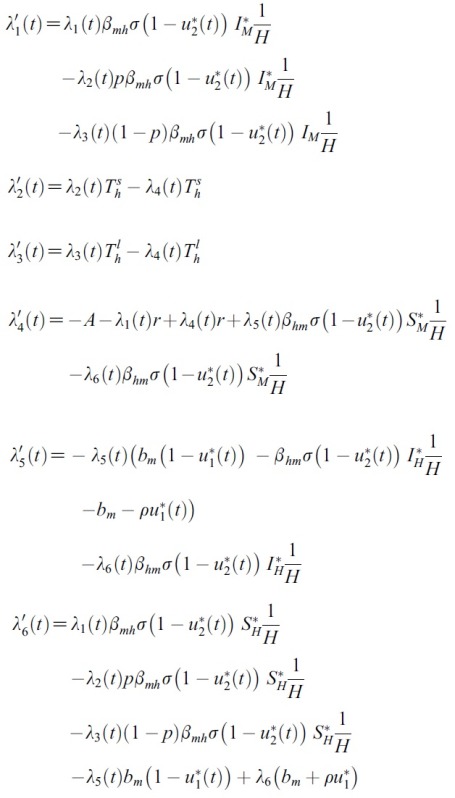
- for the optimal control problem (1) and (2). Then, there exist adjoint variables λ1(t), λ2(t), λ3(t), λ4(t), λ5(t) and λ6(t). and λ6(t) that satisfy
- with transversality conditions(or boundary conditions)
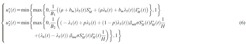
- Furthermore, the optimal control
- and
- are given by
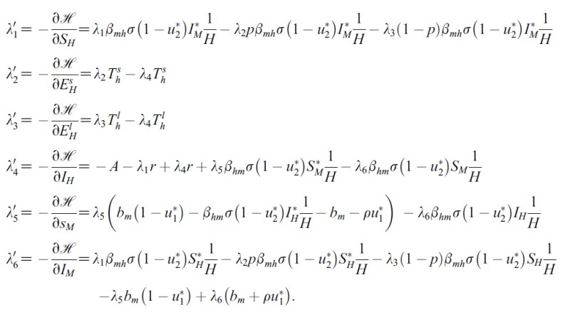
- Proof. To determine the adjoint equations and the transversality conditions, we use the Hamiltonian (4). From setting
- and also differentiating the Hamiltonian (4) with respect to SH, EsH, ElH, IH, SM and IM, we obtain
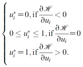
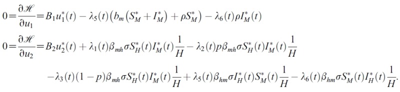
- By the optimality conditions, we have
- Using the property of the control space, we obtain the characterizations of
- and
- in (6). From the fixed of start time, we have transvesality conditions (5).
3. Discussion and Conclusions


-
Acknowledgements
- This research was supported by Kyungpook National University Research Fund 2011, and Kyeongah Nah is supported by European Research Council Starting Grant 259559, and TAMOP-4.2.2/B-10/1-2010-0012.
- 1. Feighner BH Pak SI Novakoski WL et al.. Reemergence of Plasmodium vivax malaria in the Republic of Korea. Emerg Infect Dis Apr-Jun;1998;4(2). 295−7. PMID: 9621202.ArticlePubMedPMC
- 2. Ree HI. . Studies on Anopheles sinensis, the vector species of vivax malaria in Korea. Korean J Parasitol 9;2005;43(3). 75−92. PMID: 16192749.ArticlePubMedPMC
- 3. Ross R. . The prevention of malaria.. Murray; London: 1911. 2nd ed.
- 4. MacDonald G. . The epidemiology and control of malaria.. Oxford University Press; London: 1957.
- 5. Okosun KO Ouifki R Marcus N. . Optimalcontrol analysis of amalaria disease transmission model that includes treatment and vaccination with waning immunity. Biosystems 11;2011;106(2-3). 136−45. PMID: 21843591.ArticlePubMed
- 6. Lashari AA Zaman G. . Optimal control of a vector borne disease with horizontal transmission. Nonlinear Anal: Real World Appl 2;2012;13(1). 203−12.Article
- 7. Blayneh KW Gumel AB Lenhart S et al.. Backward bifurcation and optimal control in transmission dynamics of West Nile virus. Bull Math Biol 5;2010;72(4). 1006−28. PMID: 20054714.ArticlePubMed
- 8. Blayneh KW Cao Y Kwon H-D. . Optimal control of vector-borne diseases: treatment and prevention. Discrete Contin Dyn Syst B 2009;11:587−611.Article
- 9. Bowman C Gumel AB van den Driessche P et al.. A mathematical model for assessing control strategies against West Nile virus. Bull Math Biol 9;2005;67(5). 1107−33. PMID: 15998497.ArticlePubMed
- 10. Pongsumpun P Tang IM. . Mathematical model for the transmission of P. falciparum and P. vivax malaria along the Thai-Myanmar border. Int J Biol Life Sci 2007;3(3). 200−7. Summer.
- 11. Nah K Kim Y Lee JM. . The dilution effect of the domestic animal population on the transmission of P. vivax malaria. J Theor Biol 9;2010;266(2). 299−306. PMID: 20619273.ArticlePubMed
- 12. Hartman P. . Ordinary differential equations.. John Wiley & Sons; New York: 1964.
- 13. Kelley E Petterson A. . The theory of differential equations: classical and qualitative.. Pearson Education, Inc; 2004.
- 14. Lukes DL. . Differential equations: classical to controlled. In: Mathematics in science engineering, vol. 162. Academic Press; New York: 1982.
- 15. Kamien MI Schwartz NL. . Dynamic optimization: the calculus of variations and optimal control in economics and management.. North-Holland; Amsterdam: 1991.
- 16. Lenhart S Workman JT. . Optimal control applied to biological models. In: Mathematical and computational biology series.. Chapman & Hall/CRC Press; London/Boca Raton: 2007.
- 17. Sethi SP Thompson GL. . Optimal control theory - applications to management science and economics.. Springer; 2000.
- 18. Pontryagin LS Boltyanskii VG Gamkrelidge RV et al.. The mathematical theory of optimal processes.. John Wiley and Sons; New York: 1962.
Figure & Data
References
Citations
Citations to this article as recorded by 
- Numerical Investigation of Malaria Disease Dynamics in Fuzzy Environment
Fazal Dayan, Dumitru Baleanu, Nauman Ahmed, Jan Awrejcewicz, Muhammad Rafiq, Ali Raza, Muhammad Ozair Ahmad
Computers, Materials & Continua.2023; 74(2): 2345. CrossRef - New Trends in Fuzzy Modeling Through Numerical Techniques
M. M. Alqarni, Muhammad Rafiq, Fazal Dayan, Jan Awrejcewicz, Nauman Ahmed, Ali Raza, Muhammad Ozair Ahmad, Witold Pawłowski, Emad E. Mahmoud
Computers, Materials & Continua.2023; 74(3): 6371. CrossRef - Optimal control analysis of hepatocytic-erythrocytic dynamics of Plasmodium falciparum malaria
Titus Okello Orwa, Rachel Waema Mbogo, Livingstone Serwadda Luboobi
Infectious Disease Modelling.2022; 7(1): 82. CrossRef - Effects of climate change on Plasmodium vivax malaria transmission dynamics: A mathematical modeling approach
Jung Eun Kim, Yongin Choi, Chang Hyeong Lee
Applied Mathematics and Computation.2019; 347: 616. CrossRef - Optimal bed net use for a dengue disease model with mosquito seasonal pattern
Bruno Buonomo, Rossella Della Marca
Mathematical Methods in the Applied Sciences.2018; 41(2): 573. CrossRef - Optimal control in epidemiology
Oluwaseun Sharomi, Tufail Malik
Annals of Operations Research.2017; 251(1-2): 55. CrossRef - A new analysis of infection dynamics: multi-regions discrete epidemic model with an extended optimal control approach
Omar Zakary, Mostafa Rachik, Ilias Elmouki
International Journal of Dynamics and Control.2017; 5(4): 1010. CrossRef - On the analysis of a multi-regions discrete SIR epidemic model: an optimal control approach
Omar Zakary, Mostafa Rachik, Ilias Elmouki
International Journal of Dynamics and Control.2017; 5(3): 917. CrossRef - Bifurcation and Sensitivity Analysis of Malaria–Schistosomiasis Co-infection Model
E. A. Bakare, C. R. Nwozo
International Journal of Applied and Computational.2017; 3(S1): 971. CrossRef - Effect of awareness programs and travel-blocking operations in the control of HIV/AIDS outbreaks: a multi-domains SIR model
Omar Zakary, Abdelilah Larrache, Mostafa Rachik, Ilias Elmouki
Advances in Difference Equations.2016;[Epub] CrossRef - Transmission Dynamics and Optimal Control of Malaria in Kenya
Gabriel Otieno, Joseph K. Koske, John M. Mutiso
Discrete Dynamics in Nature and Society.2016; 2016: 1. CrossRef - Years of Epidemics (2009–2011): Pandemic Influenza and Foot-and-Mouth Disease Epidemic in Korea
Hae-Wol Cho, Chaeshin Chu
Osong Public Health and Research Perspectives.2013; 4(3): 125. CrossRef
 PubReader
 Cite
Cite


